Three post-training losses, one quantity

What is preference optimization? Every once in a while ChatGPT asks me if I prefer response A or response B. When I look at the two responses, I think about whether there’s actually a difference in the content or just in how it’s presented. When you Google something, multiple results come back. Some are what I’m looking for, others are outright wrong. With the options ChatGPT comes back with, I don’t know that either is outright wrong. But beyond stylistic differences, one might go deeper into one confusion point while the other goes deeper into a different one.

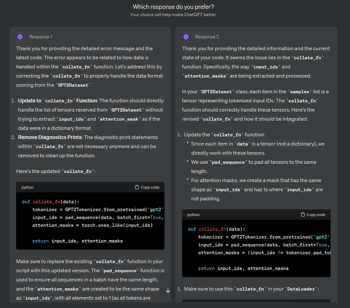A ChatGPT "which response do you prefer" prompt Figure 1. In this example the difference appears stylistic.

How does my preference inform how ChatGPT should talk to me? How does my preference of the sequence of words map its way back to how the model chooses which tokens to output?

Is there an optimal style of english for me, tuned to the words and concepts I already hold, that transfers the most information in the fewest words? And past style, is there an optimal breakdown of a new idea into pieces isomorphic to things I already understand?

To begin answering any of that, I first need to understand how a preferred response changes the model’s next-token probabilities, which means understanding the losses driving the change. The popular post-training methods are SFT (imitate demonstrations), DPO (learn from preference pairs, the A/B preference above), and GRPO (learn from groups of attempts scored by a verifier). These are three ways of consuming one quantity. That quantity is $\log\pi(y\mid x)$ , the log-probability the model assigns to a given response.

The one quantity, $\pi(y\mid x)$

$\pi(y\mid x)$ is the probability that the model assigns to response $y$ , given prompt $x$ . Not the probability of the best response, or of a response. It is the probability of one, fully specified sequence of tokens. Every loss is built out of logs of this number and nothing else.

The symbol is doing three jobs here. The network (token ids in, logits out), the distribution $\pi(\cdot\mid x)$ (which is never materialized) and the scalar $\pi(y\mid x)$ , the distribution evaluated at one given response. Jobs 1 and 3 are related but not identical. The network is the machine. One forward pass of it, plus a log-softmax, a gather at the label’s token ids, and a sum, produces the scalar. Job 3 is a single reading taken from the job-1 machine, and it’s recomputed from the current weights at every training step. Token ids come from the dataset. Probabilities never do.

What would the distribution look like if you could materialize it? A table with one row per possible response:

response $y$ (a full sequence)	$\pi(y \mid x)$
” Paris.”	0.0031
” Paris, the capital of France.”	0.0007
” purple monkey dishwasher”	0.0000000002
… one row per possible sequence …	…

Probabilities illustrative.

How many rows? For GPT-2’s vocabulary ( $V = 50{,}257$ ) and a 9-token response, $V^L = 50257^9 \approx 10^{42}$ rows. That’s why the table is never built, and why the only thing we ever compute is one row’s value via forward pass.

All losses take logpis, $\log\pi(\cdot\mid x)$ . Compactly, $\pi$ is a stand-in for a policy. In traditional RL, a policy looks at a state and assigns probabilities to actions. Here, the whole prompt collapses into one state $x$ , and one whole response collapses into one action $y$ . An action in this view is an entire response, one draw out of the $V^L$ candidates, not a single next-token pick. (The per-token view comes back in Bug 2.) The policy spreads its probability across all $V^L$ candidates, $\pi(y\mid x)$ is the share assigned to the one action we care about, and $\log\pi(y\mid x)$ is its log. One scalar per (prompt, response) pair. Training moves probability mass toward better actions. The log changes nothing about the ranking (it’s monotonic), and it’s there because it turns the chain-rule product over tokens into a sum.

With that scalar, the first loss is immediate. Take an actual label $y$ from the dataset and ask what probability the model gave the label we actually got. You want that number large, so you want its negative log small. That’s SFT.

Ten lines of Python

def sft_loss(logpi):
    return -logpi

def dpo_loss(logpi_c, logpi_r, ref_c, ref_r, beta=0.1):
    exp = beta * ((logpi_c - ref_c) - (logpi_r - ref_r))
    return -torch.nn.functional.logsigmoid(exp)

def grpo_advantages(rewards):
    return (rewards - rewards.mean()) / (rewards.std(correction=0) + 1e-8)

def grpo_loss(logpis, advantages):
    return -(1/len(advantages)) * torch.dot(logpis, advantages)

To make things concrete, let’s use toy numbers. Two models are in play. The policy $\pi_\theta$ is the model being trained. The reference $\pi_{\text{ref}}$ is the frozen checkpoint training starts from, and at step 0 the two are identical. One preference pair, scored by both, as if you’re the annotator looking at the two options side by side:

	chosen $y_w$	rejected $y_l$
$\log\pi_\theta(y\mid x)$ (policy)	$-12.3$	$-15.7$
$\log\pi_{\text{ref}}(y\mid x)$ (reference)	$-13.1$	$-14.9$

And one GRPO group, four sampled responses to the same prompt with verifier rewards $[1, 0, 0, 1]$ , which standardize to advantages $[1, -1, -1, 1]$ exactly (mean $.5$ , population std $.5$ ). The verifier here returns binary right/wrong, which suits checkable domains like math and code, but GRPO doesn’t require binary rewards. It only needs some scalar per response. A reward model trained on human preferences works too, handing back a continuous score, and DeepSeekMath uses both. A noisy or inconsistent judge makes the advantages noisy. A hackable one gets hacked.

Three bugs, three rules

Bug 1: I put the log in the wrong place

# context: inside dpo_loss(logpi_c, logpi_r, ref_c, ref_r) above.
# logpi_c / ref_c = the chosen response's log-prob under the policy / the reference.

y_w_ratio = logpi_c / ref_c                                  # attempt 1: divided two LOG values
exp = beta*torch.log(y_w_ratio) - beta*torch.log(y_l_ratio)  # attempt 2: logged a log-ratio -> log(0) -> nan

# what the DPO objective actually says:
exp = beta * ((logpi_c - ref_c) - (logpi_r - ref_r))         # ratio in prob-space = SUBTRACTION in log-space

It had to do with deriving the formula. I missed that the log was actually on the outside of the ratio, not all the way on the inside. The same shape showed up in my handwritten notes that weekend:

\mathbb{D}_{\text{KL}}(\pi \,\|\, \pi_{\text{ref}}) = \mathbb{E}\left[\frac{\log \pi}{\log \pi_{\text{ref}}}\right] \quad\text{(what I wrote)} \qquad\text{vs.}\qquad \mathbb{E}\left[\log \frac{\pi}{\pi_{\text{ref}}}\right] \quad\text{(the definition)}

The log of a ratio is completely fine. The DPO loss is one. The banned shape is a ratio of logs. The rule: a product in probability-space is a sum in log-space, and a ratio in probability-space is a subtraction in log-space.

Bug 2: I dropped the minus sign

Here is the DPO objective itself (equation 7 of the DPO paper), the thing the code implements:

\mathcal{L}_{\text{DPO}} = -\,\mathbb{E}_{(x,y_w,y_l)\sim\mathcal{D}}\left[\log \sigma\!\left(\beta\log\frac{\pi_\theta(y_w\mid x)}{\pi_{\text{ref}}(y_w\mid x)} - \beta\log\frac{\pi_\theta(y_l\mid x)}{\pi_{\text{ref}}(y_l\mid x)}\right)\right]

return torch.nn.functional.logsigmoid(exp)    # what I wrote
return -torch.nn.functional.logsigmoid(exp)   # the objective

I thought the formula with the negative sign in front was the likelihood, so to maximize the likelihood we want to minimize the opposite, and since we usually want to minimize a loss, I dropped the negative term.

The rule: maximizing the likelihood function = minimizing the negative version. The minus is what manufactures a minimizable object. (Part of the trap is that in ML, $\mathcal{L}$ canonically means loss, the negative log-likelihood, already minimize-ready. The statistician’s likelihood also uses $\mathcal{L}$ . Same letter, opposite optimization direction.)

While catching this I hit a second mixup. MLE is maximizing $P(\mathcal{D}\mid\theta)$ , finding the model params $\theta$ under which the data we saw is maximally probable. But which product is being maximized? I could see three candidates and was confused which one the loss corresponded to:

\prod_{\mathcal{D}} P(y_w \mid x) \qquad\text{or}\qquad \prod_t P(y_t \mid x, y_{<t}) \qquad\text{or}\qquad \prod_{\mathcal{D}} \sigma\big(r(x,y_w) - r(x,y_l)\big)\;?

In words. The first goes through the whole dataset and multiplies the probability of each winning response. The second goes through one response and multiplies each next-token probability. The third goes through the whole dataset and multiplies the Bradley–Terry probability of each observed win.

They nest at three levels:

\mathcal{L}_{\text{DPO}} = -\underbrace{\sum_{(x,\,y_w,\,y_l)\,\in\,\mathcal{D}}}_{\text{level 1: dataset}} \log\; \underbrace{\sigma\big(r_\theta(x,y_w) - r_\theta(x,y_l)\big)}_{\text{level 2: one BT preference per pair}}

\log\pi_\theta(y\mid x) = \underbrace{\sum_t \log p_\theta(y_t \mid x, y_{<t})}_{\text{level 3: chain rule, inside each log-prob}}

The glue between the levels, explicitly. Level 3 sums token log-probs into one $\log\pi(y\mid x)$ . Two of those, policy minus reference for the same response, make one implicit reward, $r_\theta(x,y) = \beta\log\pi_\theta(y\mid x) - \beta\log\pi_{\text{ref}}(y\mid x)$ . Two implicit rewards, chosen minus rejected, make the margin that level 2’s $\sigma$ converts into a win probability. Level 1 sums the log of that probability over every pair in the dataset. That chain is how a token-level quantity ends up inside a preference-level loss.

Concretely, with the running example. Level 1 ranges over all the A/B clicks ever collected. Level 2 is one click, say preferring ” Paris.” over ” purple monkey dishwasher”. Level 3 is the token-by-token probability of ” Paris.” itself.

My confusion was trying to make one product do all three jobs. And the minus sign ties it off. Minimizing without it would train the judge to find the observed winners maximally unlikely, which is a model that prefers the rejected response.

Bug 3: I deleted the epsilon in GRPO

return (rewards - rewards.mean()) / rewards.std(correction=0)          # what I wrote
return (rewards - rewards.mean()) / (rewards.std(correction=0) + 1e-8) # the spec

I added torch.finfo(torch.float16).eps as the epsilon and my test failed due to precision. So I dropped the epsilon entirely, and every test still passed.

Here’s the failure that the tests never fed it. Prompt: “What is the capital of France?” Sample $G = 4$ responses. All four say Paris, so the verifier returns $[1,1,1,1]$ . All-equal groups are routine in real training, because easy prompts saturate (and hard ones return all zeros). Now the mean is 1, the std is 0, and the z-score formula $(r_i - \bar r)/\text{std}$ divides by zero. Four NaNs, batch poisoned. What we actually want is $[0,0,0,0]$ , because a group with no spread carries no learning signal. That’s the rule: the epsilon is not precision fuzz, it’s a zero-signal guard.

Why $10^{-8}$ specifically (the 1e-8 in the code)? Convention. It needs to be small enough to leave any real std untouched. The smallest nonzero std for binary rewards in a group of four is $\approx 0.43$ (one 1 among three 0s gives mean $.25$ , deviations $\{.75, -.25, -.25, -.25\}$ , mean square $.1875$ , square root $\approx .43$ ). And it needs to be large enough that $0/\varepsilon$ is a clean zero. $10^{-8}$ clears both bars with room to spare. It’s also the same default $\varepsilon$ Adam uses.

The judge and the sampler

A question the drill forced me to predict before running: what is the DPO loss when policy == reference, exactly? Policy == reference means the two models agree at every response, $\log\pi_\theta(y\mid x) = \log\pi_{\text{ref}}(y\mid x)$ for all $y$ . This is literally the situation at training step 0, since the policy is initialized as a copy of the reference. Working through BT I got to $\sigma(0) = \tfrac12$ , and then misread what the $\tfrac12$ meant. My first reading was that $\tfrac12$ is the probability of the current model outputting $y_w$ vs $y_l$ .

A check with the toy numbers kills that reading. Force the model to choose between just the two responses in our table. The two-way choice probability is the renormalized share, and the algebra collapses to a sigmoid of the log-prob difference:

P(\text{emit } y_w \text{ over } y_l) = \frac{\pi(y_w\mid x)}{\pi(y_w\mid x) + \pi(y_l\mid x)} = \sigma\big(\log\pi(y_w\mid x) - \log\pi(y_l\mid x)\big) = \sigma(-12.3 + 15.7) = \sigma(3.4) \approx 0.97

So even at policy == reference, the model already prefers to emit the chosen response 97 to 3. The $\tfrac12$ cannot be about emission. It is the probability of a different event, judged by a different machine.

Two machines live in one network. The sampler scores emission, “how likely am I to say this?” That’s the $0.97$ , and it comes from the raw log-probs. The judge scores movement. Its score for one response is the implicit reward $\beta\log\frac{\pi_\theta(y\mid x)}{\pi_{\text{ref}}(y\mid x)}$ , which asks one question. Has training raised this response’s probability above where the reference left it? At step 0 the answer is no for every response, by construction. The policy is the reference, the ratio inside the log is 1, and $\beta\log 1 = 0$ . Every implicit reward is exactly zero, so the judge has no basis to prefer either response and sits at chance, $\sigma(0 - 0) = \tfrac12$ . The loss per pair at that moment is $-\log\tfrac12 = \log 2 \approx 0.693$ .

That number is worth keeping as a landmark, and pretraining has the same kind. A freshly initialized model spreads probability uniformly over the vocabulary, each token gets $1/V$ , and the per-token loss is $-\log(1/V) = \log V$ . Every training regime has a loss value that means “nothing learned yet.” $\log V$ is pretraining’s. $\log 2$ is DPO’s.

Where does the judge’s formula come from? Bradley–Terry (BT) is the judge, a model of the probability that $y_w$ is preferred to $y_l$ . Assume there’s an actual reward function $r^*$ that can score $r^*(x,y_w)$ and $r^*(x,y_l)$ . A tempting first guess for the judge’s probability is a raw ratio of the rewards,

P(y_w \succ y_l \mid x) = \frac{r(x,y_w)}{r(x,y_w) + r(x,y_l)} \quad\text{(broken)}

but that breaks. Reward can be any real number (try a negative one) and probabilities need to be $0\to 1$ . So take exponents first, and if we massage that we actually just get sigmoid of the difference of the rewards:

P(y_w \succ y_l \mid x) = \frac{e^{r(x,y_w)}}{e^{r(x,y_w)} + e^{r(x,y_l)}} = \sigma\big(r(x,y_w) - r(x,y_l)\big)

Note this is the same two-way softmax algebra as the emission check above. The only difference is what plays the role of the score. Log-probs as scores give the sampler. Rewards as scores give the judge.

So we’re taking the difference of the rewards of choosing $y_w$ and $y_l$ and squeezing it exponentially into $0\to 1$ . The bigger $y_w$ ‘s reward edge, the closer the judge probability is to 1. The smaller the difference, the closer to 0.5 (random). If the difference is negative, meaning $y_l$ has the higher reward, the judge probability drops below 0.5 and $y_w$ is not gonna win against $y_l$ .

Now remember how we said $r^*$ is a given oracle. In reality we have to estimate it. Call the estimated reward model $r_\phi$ . Since we already have the preference data, we know what the judges picked between $y_w$ and $y_l$ , so we can learn parameters $\phi$ that make those choices maximally likely. This is how reward models get trained. (To be clear, this is not SFT. SFT imitates demonstrations and never sees preferences.)

But actually, why don’t we try seeing if we can ditch the reward model altogether? The trick is to define an optimal policy $\pi^*$ directly from the reference and the reward,

\pi^*(y\mid x) = \frac{1}{Z(x)}\,\pi_{\text{ref}}(y\mid x)\,e^{\,r(x,y)/\beta},

and then invert it, which expresses the reward in terms of policies instead of the other way around:

r(x,y) = \beta\log\frac{\pi^*(y\mid x)}{\pi_{\text{ref}}(y\mid x)} + \beta\log Z(x).

Plug that into BT’s difference and the unknowable $Z(x)$ cancels, leaving a loss with no explicit reward model in it. What survives the substitution is BT’s real gift, a proper likelihood for pairwise data. Concretely. The dataset says $y_w$ beat $y_l$ , and the model replies “I give that outcome probability $\sigma(r_w - r_l)$ .” Multiply those over every comparison in the dataset and you get the probability of everything you observed, as a differentiable function of the parameters. That one number is what MLE climbs. Without a likelihood you could only count wins, and counts don’t transfer. With one, every comparison anywhere in the dataset pushes the same underlying parameters, and the fitted reward can score pairs it never saw.

Chess Elo is Bradley–Terry, with players for responses, games for comparisons, and ratings for rewards. From sparse pairwise games it produces one rating per player that predicts matchups never played. Same here. Every A/B click sharpens the implicit reward everywhere, and with enough clean pairs it converges to the true one, up to a per-prompt constant. (Why $\pi^*$ deserves the word optimal rather than just being a name is a gorgeous trick. It uses optimality conditions as relations between unknowns rather than equations to solve, the same move that powers Lagrangian duality.)

Why DPO needs a reference, GRPO needs a group, and SFT needs neither

DPO compares the current policy against another policy, the reference. GRPO compares across samples. SFT compares to the actual data that’s been seen.

A tempting objection. Doesn’t every post-training method start from some checkpoint, so don’t they all “need a reference”? Distinguish initialization from participation. Starting from a checkpoint is initialization, and yes, everyone does it. SFT initializes from the base model and then the base never appears in its loss. After the first step you could delete it. DPO’s reference is different. It participates in the loss, a second forward pass on every example, at every training step, forever, because the implicit reward is defined as movement away from it. That’s also why DPO needs no verifier (the humans already judged, the pairs are the supervision) and no value function (there’s no sampling loop to tame, it’s classification on fixed pairs).

Doesn’t GRPO also have a KL term to the reference? It does, but look at where the reference lives in each loss, side by side:

\mathcal{L}_{\text{DPO}} = -\log\sigma\Big(\beta\big[\underbrace{(\log\pi_\theta(y_w\mid x) - \log\pi_{\text{ref}}(y_w\mid x))}_{\pi_{\text{ref}}\text{ inside the reward itself}} - (\log\pi_\theta(y_l\mid x) - \log\pi_{\text{ref}}(y_l\mid x))\big]\Big)

\mathcal{L}_{\text{GRPO}} = \underbrace{-\frac{1}{G}\sum_{i=1}^{G} A_i \log\pi_\theta(y_i\mid x)}_{\text{complete loss on its own}} \;+\; \underbrace{\beta\,\mathbb{D}_{\text{KL}}\big(\pi_\theta \,\|\, \pi_{\text{ref}}\big)}_{\text{separate, detachable term}}

In GRPO the reference sits in its own added term. Set $\beta$ to zero, snip it off, and a valid training algorithm remains (the simplified version above has no reference anywhere and passes its tests). In DPO the reference is inside the sigmoid’s argument. Delete it and you no longer have a pulse on the reward, because the implicit reward is defined against the reference. There’s no loss left to compute. (PPO, for contrast, hides its KL as a per-token penalty folded into the reward. GRPO’s move was making it an explicit, separable loss term.) Delete GRPO’s and you merely risk policy drift. It samples from itself, and without the leash it can wander into reward hacking. A worse model, but still a well-defined loss.

GRPO doesn’t need a value network because the value can be inferred empirically, as a Monte Carlo estimate from the $G$ outputs. You need a group because to estimate, you need multiple samples. (An open question I’m parking. What are the sample-complexity bounds here, i.e. how big does $G$ really need to be? DeepSeekMath uses $G = 64$ .)

And imitating demonstrations needs neither a baseline nor a reference because you know the exact output tokens you are trying to imitate, and you hill-climb against those directly. (Another parked wondering. Is the “transfer of bits” of intelligence bounded differently between direct SFT and the softer, latent transfer of preference optimization? That’s the signal ladder below, asked quantitatively.)

The signal ladder

The core tension is connecting RL to supervised learning, and Bradley–Terry is the angle, supervision via direct preference comparison. DPO deletes the moving-data property. (Moving data means the training distribution shifts as the policy updates, because the policy generates its own training samples. A frozen set of preference pairs doesn’t move.) The closed form solves the sampling loop on paper, leaving supervised learning on a fixed dataset. The price is that it’s off-policy, trained on pairs collected once from whatever model generated them. GRPO keeps the sampling loop, fresh samples from the current policy every batch, on-policy, which is why it’s still RL.

So what does each loss actually get per example? SFT gets the exact output for a prompt and trains the model toward it directly. The densest signal, a target at every token, but capped at imitation. DPO gets a preference pair and learns to edge toward the winner, implicitly aligned with the underlying reward by construction, a leashed $\pi_{\text{ref}}$ with favorability toward the reward. One bit per pair. GRPO gets a group of $G$ outputs and constructs advantages from the reward. “Monte Carlo estimate” sounds fancier than it is. The margin-note version: average the $G$ rewards, and that average is “how good a typical response to this prompt is,” the prompt’s value, measured instead of learned. Subtracting it asks each sample one question. Are you better than your siblings? That’s the sparsest signal per sample, but on-policy and verifier-grounded, so it’s the only one of the three that can climb past its data.

One last trap. In practice we watch the reward curve, not the loss curve, and not only because an all-equal group has nothing to teach (advantages 0). (Pleasingly, the same is true of human learning. Practice material you always get right, or always get wrong, carries no gradient for you either. Aim for the edge. That idea is its own future post.) The GRPO loss hovers near zero for EVERY group, by construction. Standardized advantages are mean-zero, so the expected loss is pinned at $\approx 0$ at any skill level, even while real learning happens underneath. The gradients are alive, only the expectation is pinned. The loss value carries no progress signal. The reward curve is the only one that trends.

Next up, real numbers. A (prompt, chosen, rejected) triple through GPT-2 and an actual DPO margin. The full ratio/clip/KL GRPO is its own future post.

The one quantity, π(y∣x)\pi(y\mid x)π(y∣x)